How I stopped worrying and learned to fetch, aggregate, and reshape AFL player data.

Jupyter notebooks used for this post can be found here.
When I started this project, one of my main goals was to incorporate player data into my footy-tipping model. Footy Tipper, my model for last season, incorporated betting and team-match data into an ensemble, but I couldn’t quite figure out how to include player-based features in a way that enhanced performance. I tried sorting player lists alphabetically, treating player names like categorical variables, then adding embedding layers to my neural net, but that just added noise and actually lowered accuracy slightly. I didn’t have much time to experiment, as the AFL season was quickly approaching, so I dropped the idea of using player lists for the time being, vowing to return with more men, horses, and steel. With the advent of Tipresias, I’m making another assault on the barricades with a few new weapons at my side.
fitzRoy is good, but I’m a pythonista
During the recent AFL season, I started looking into the robust AFL stats community that I, in my American chauvinism, had assumed didn’t exist. What? A regional professional sports league in a country with 7.6% of the population of the U.S. is big enough to support a slew of data-crazed fans capable of writing sufficient blog posts and tweets to inform my new-found interest in footy stats? Consider me humbled. I followed a few accounts on Twitter, read some posts on Matter of Stats, HPN, and started comparing my model’s performance to those of the notables competing on Squiggle.
In addition to teaching me about the finer points of footy, my research yielded this little gem: fitzRoy. fitzRoy is an R package that scapes popular AFL stats sites, cleans the data, and serves up data frames on the good china. It even has decent documentation! I was quite excited at the prospect of getting tons of data with minimal effort, because using an open-source package is way easier than maintaining my own website scraper, especially when faced with the borgesian nightmare that is navigating AFL Tables. The only problem is that I do all my work in Python, and fitzRoy is strictly for R, the basics of which I learn every couple of years, then promptly forget from lack of practice. I have a great data source in R; I have a data-consuming, machine-learning model in Python; how on earth do I get the twain to meet?
Luckily, there’s a tool for everything, even tools for getting your tools to work better. A little googling led me to the Python package rpy2, whose entire purpose is to let you run R in a Python context, whether that means importing R packages as Python modules, running your own R code directly in a .py file, or converting R data frames to pandas. Unfortunately, this adds an extra level of complication to my project dependencies: not only am I using a few more packages, but I now need two full languages available in my development environment. The best tool for solving this problem is definitely Docker (with code, it’s tools all the way down), especially if you plan on running code like this on different machines or collaborating with others. This isn’t a Docker tutorial (if you’re interested, you can can check out the Docker setup for Tipresias on GitHub), but the basic idea is that it creates an isolated virtual environment (i.e. a ‘container’) in which you can run your code. This means that you can install exact versions of all of your dependencies without worrying about conflicts with other libraries on your computer. Also, a collaborator can easily create a development environment with everything already installed by just entering a few commands.
I had not thought that footy had undone so many
Over 121 years, a lot of people have played a lot of matches in the VFL and AFL: 619,751 (plus a hundred or so from a few round-robin rounds that were easier to drop than munge), give or take. The size of this data set presented new challenges that went beyond longer processing times. For one, my Jupyter notebook kept crashing while I was cleaning and transforming the data, which caused me to spend a whole weekend figuring out how to do it in batches only to realise that all I needed was to increase Docker’s memory limit.
As for figuring out how to get the player data into a useful shape for match predictions, in the spirit of always starting with an MVP (‘minimum viable product’ in this context), I settled on a simple approach: calculate a rolling mean of each player’s stats (e.g. kicks, marks, goals), then add up the mean stats for all the players on a given team who participated in a given match. This functions similarly to using a rolling mean of a team’s in-game stats, but with the added nuance of only including the recent performance of players who are actually playing. So, if a team’s best player is not playing in their next match, the aggregated stats will reflect this diminishment in the team’s expected performance.
Getting a model on the board
Now that I have my player data aggregated and organised into team-match rows, like the datasets for my other models, I can start looking at the relative performance of various machine-learning models. As with models based on other datasets, I found that including both a team’s stats and their opponent’s stats improves model performance, with the lowest cross-validation mean absolute error (MAE) being 31.79 without opposition stats and 30.95 with those stats. Below are the MAEs for various models using aggregated player data for teams and their opponents.
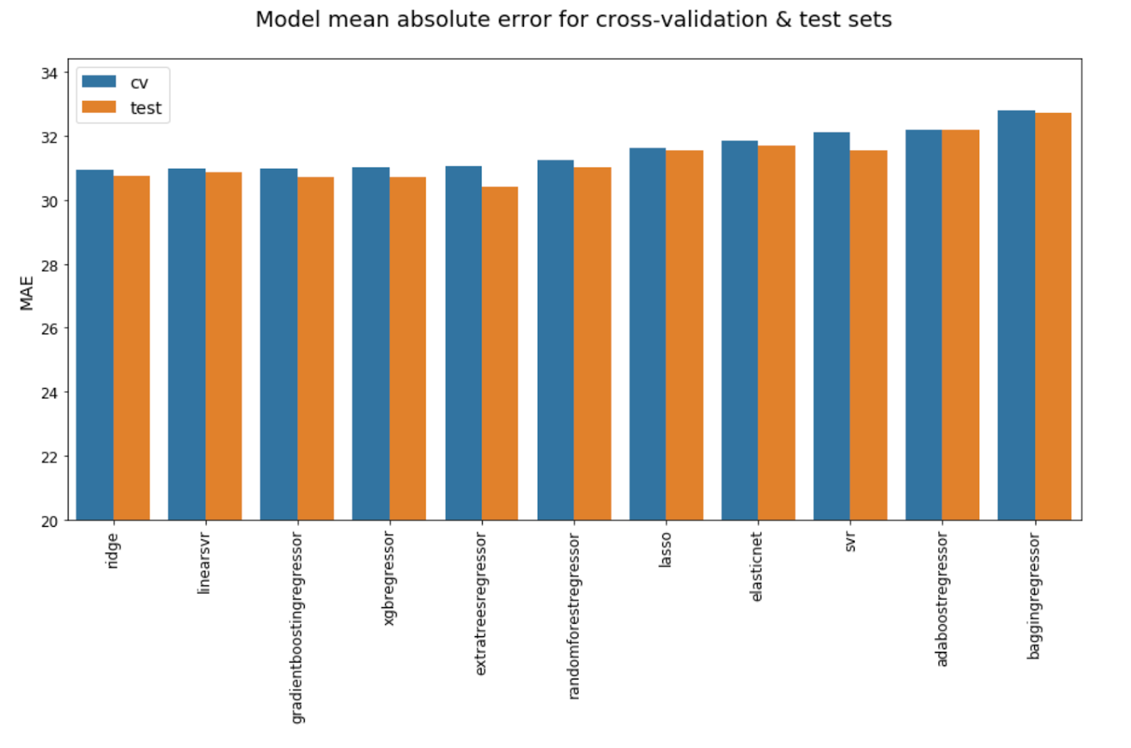
As with the betting data, though less pronounced this time, linear models are outperforming the fancy ensembles. However, the top five are all so close that if they weren’t in ascending order, it would be difficult to pick the best. The accuracy scores below further demonstrate just how close these models’ performances are.
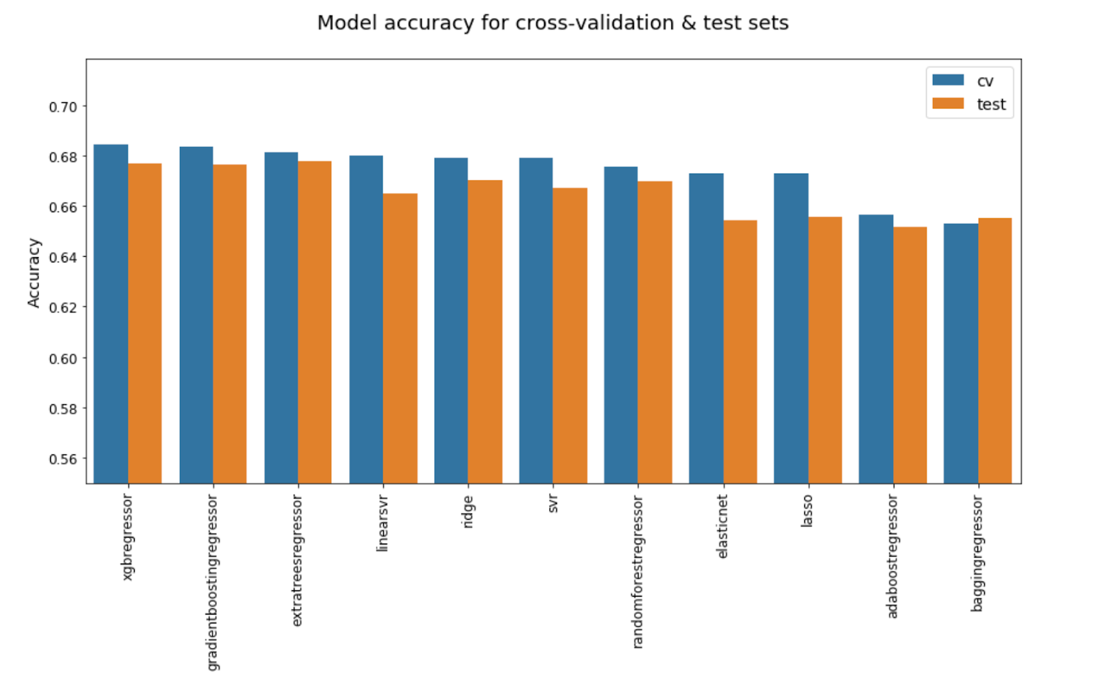
When looking at model accuracy, LinearSVR and Ridge are still toward the top, but they’re now behind the ensemble models that are third through fifth for MAE scores. Thankfully, at least the same models are in the top five for both MAE and accuracy, which limits how many I need to compare in a year-by-year breakdown of performance.
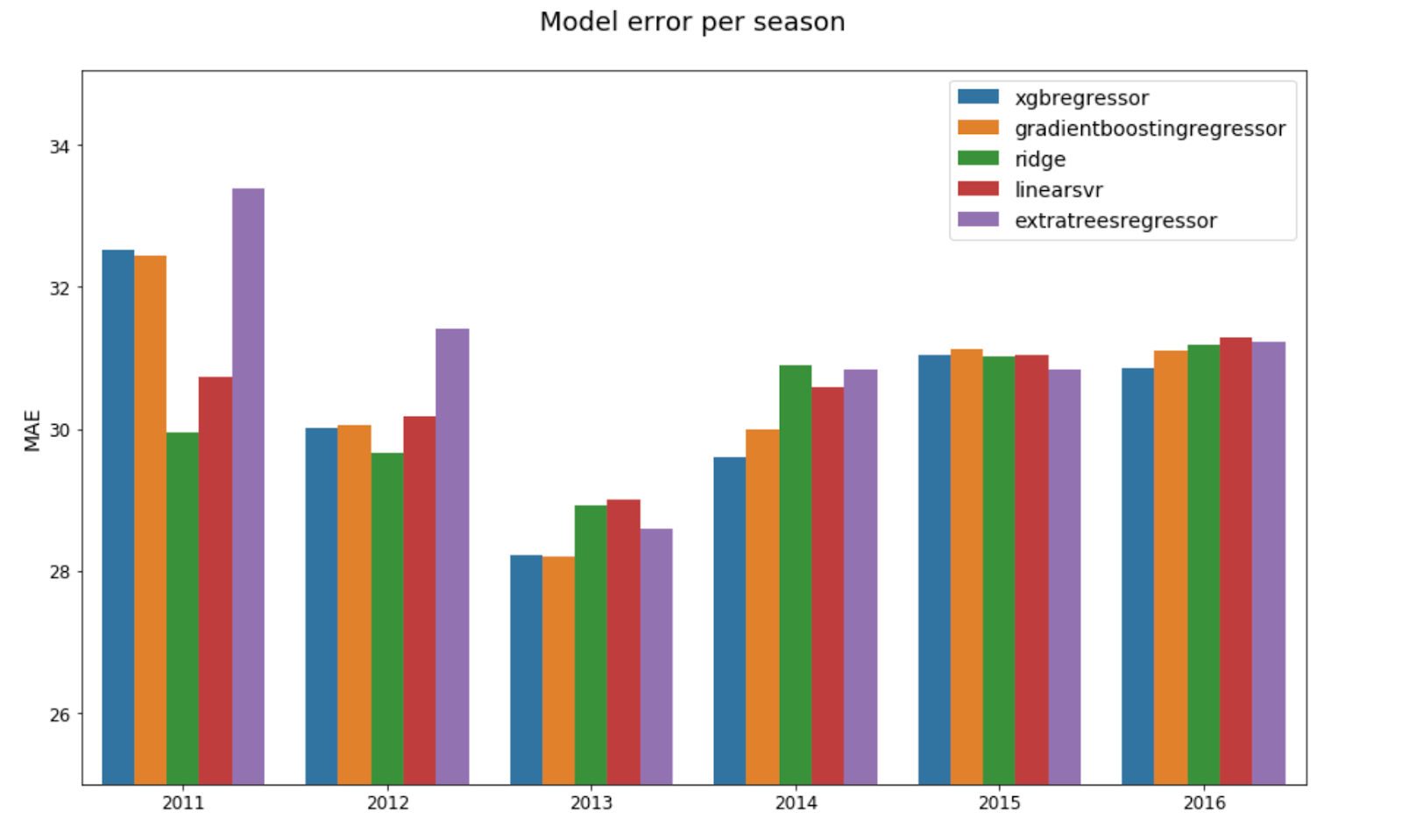
Ridge and XGBoost seem to have the best yearly MAEs, with each having the lowest in two years, but as with the CV/test scores, there isn’t a clear winner as the error scores in 2015 and 2016 are very close, and neither XGBoost nor Ridge is consistently in the top two for any given year.
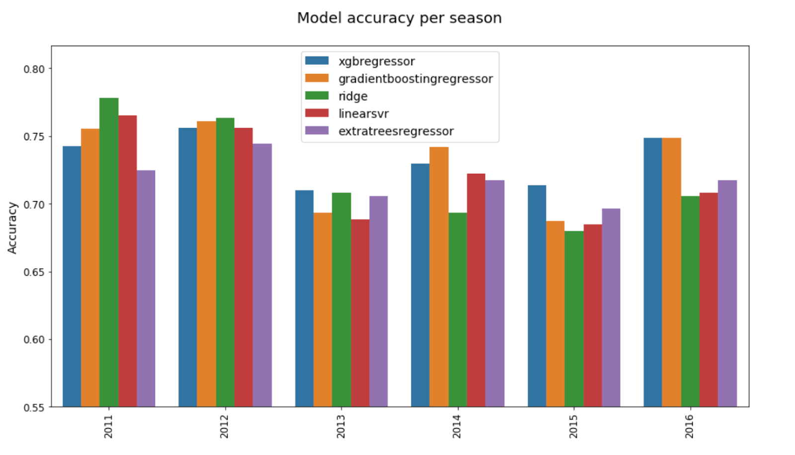
No matter how many different ways I slice the data, I keep getting mixed results. It’s a bit of a gut call at this point, but XGBoost tends to be one of the better models across different metrics and data segments. It’s not a clear winner (both Ridge and GradientBoost have roughly equal performance), but I’ve had good results from using XGBoost in the past, and that’s enough to give it the edge.
Player rating model
Inspired by HPN’s PAV, but not knowing enough about footy to apply the rigour necessary to creating my own player rating system, I wondered if I could get an algorithm to create one for me. Instead of aggregating player in-match stats as I did above, I fed them, along with some aggregated opposition stats, into a regressor to try to estimate each player’s contribution to the final score. It’s a simplistic approach, but I just wanted to see if it had any potential as a means of using player data to predict match results.
I put unaggregated player data through a few linear algorithms (when I tried to use scikit-learn ensembles, it took waaaay too long to train), to estimate the final score margin for each match based on each player’s in-game stats. I then took the best-performing model and used its predictions to create a player rating feature, which I aggregated by team by match (i.e. each match has two rows, one for each participating team) for the final model. The final performance of this stacked ensemble wasn’t too terrible, but the best-performing models still had a couple more points of MAE and a few percentage points lower accuracy than the simpler models based on aggregated player stats, and even if the relative performance were closer, the amount of time it took to train a model on raw player data was painful. Seriously, my notebook would occasionally hang midway through calculating cross-validation scores, and it it was like Sisyphus’s boulder rolling back down into the stygian depths. There is the possibility of using something like this to add a feature to the main player-data model, but I imagine I would get better performance out of adding PAV instead, so this idea is very low priority for future experimentation.
Player data in 3D
Given that player data adds an additional segment to my initial team-match data structure, I wondered if, instead of aggregating the stats, I couldn’t just break the players out into their own dimension, transforming matrices with dimensions [team-match x aggregated feature] into [team-match x player x feature]. Getting the data shape right required more work than I had hoped, but I was able to reuse some code from the recurrent neural network (RNN) in Footy Tipper to get it over the line. The biggest challenge for me is always getting the data in the correct sort order and figuring out the correct dimensions such that numpy’s reshape works the way I want it to. Once I get beyond two dimensions, my brain starts to break, but I got there eventually.
As with the player-rating model, this was just an experiment, so I implemented the simplest version possible, opting for one-dimensional convolutional layers interspersed with the usual pooling layers. Having more experience with RNNs, I was pleasantly surprised by how quickly the CNN models trained on the data, but overfitting was a major issue even with dropout or regularisation parameters. The error on the training set kept going down with each epoch while the validation error would peak two or three epochs in, then proceed to rise. This resulted in similar performance to the player-rating model, namely, at best, in the range of 30–32 for MAE and 64–66% for accuracy, both metrics being decidedly worse than linear models trained on aggregated player data. There is some potential for adding this to an ensemble or expanding the data somehow to reduce the overfitting, but for now, as with the player-rating model, this sort of experiment is a lower priority than working on other improvements, such as feature engineering and implementing an RNN on the full data set.
What have we learned today?
I feel like the refrain of this series of blog posts is “keep it simple, stupid”. Though I don’t regret spending time on experimenting with more-complicated methods, basic linear models have consistently performed as well or better than the fancy ensemble models. Even when the almighty XGBoost is the best model, there are always at least a couple of linear models that are just a hair worse and probably sometimes better when using the right random seeds. Having seen measurable gains from creating ensembles from a few different model types, however, I think the slightly more-nuanced lesson is to start with simple building blocks before moving on to constructing the whole castle. It’s important to have a good foundation against which you can compare the impact of future changes.